Kalman Filter

Problem 1 - 1D Kalman Filter

Problem Statement:

Consider a sensor that is tracking the motion of an object that is a known distance (Do = 100 m) from the sensor. Let θ_m be the angle (in radians) that is measured by the sensor.

Suppose you know that the position of the object (in meters) is governed by the following equation of motion:

X(t+1) = X(t) + w(t)

where t is measured in seconds and w(t) is a random change in the position of the object (each second) that one assumes to be normally distributed around 0 with a standard deviation of 1.0 m. The relationship between the sensor output and the actual position of the object may be characterized as follows:

θ_m (t) = X(t)/Do + v(t)

where v(t) is a random uncertainty in the measurement of θ(t) that is assumed to be normally distributed around 0 with a standard deviation of 0.010 radians.

We want to build a Kalman filter that will best predict the next location of the object and examine its characteristics with respect to the state estimation error covariance and sensor and process noise properties.

Suppose θ_m (0) = 0.000 rad, θ_m (1) = 0.010 rad, and θ_m (2) = 0.020 rad.

MATLAB Code: problem_1.m

Author: Yash Bansod
Date: 2nd May, 2020
Problem 1 - 1D Kalman Filter

GitHub: https://github.com/YashBansod

Clear the environment and the command line

clear;
close all;
clc;

Define the input parameters

init_state = 100;               % Initial state
init_cov = 0.1;                 % Initial state covariance
Q = 3;                          % System Process Noise
R = 0.0009;                     % Measurement Noise
delta_t = 1;                    % Delta time
num_steps = 51;                 % Number of time steps (including t=0)

Define the environment data

% Define the actual position of the object over time.
X_a = random('Normal', 0, 1, 1, num_steps);
X_a(1) = init_state;
X_a = cumsum(X_a);

% Define the obtained sensor measurements over time.
theta_m = (X_a / init_state) + random('Normal', 0, 0.01, 1, num_steps);
% theta_m(1) = 0;
% theta_m(2) = 0.01;
% theta_m(3) = 0.02;

% Raw conversion of sensor measurement to object state
X_m = theta_m * init_state;

Kalman Filter Variables

F = 1;
H = 1/init_state;

X_p = zeros(1, num_steps);
X_p(1) = init_state;

P_p = zeros(1, num_steps);
P_p(1) = init_cov;

X_u = zeros(1, num_steps);
X_u(1) = init_state;

P_u = zeros(1, num_steps);
P_u(1) = init_cov;

K = zeros(1, num_steps);
K(1) = (P_p(1) * H') * inv((H * P_p(1) * H') + R);

Kalman Filter Loop

for step = 2:num_steps

    % Prediction Stage
    X_p(step) = F * X_u(step - 1);
    P_p(step) = (F * P_u(step - 1) * F') + Q;

    % Update Stage
    K(step) = (P_p(step) * H') * inv((H * P_p(step) * H') + R);
    X_u(step) = X_p(step) + (K(step) * (theta_m(step) - H * X_p(step)));
    P_u(step) = P_p(step) - (K(step) * H * P_p(step));

end

Plot the results

time_line = 0:delta_t:(num_steps - 1)* delta_t;

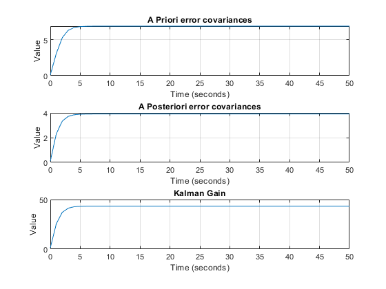
figure(1);
subplot(3, 1, 1)
plot(time_line, P_p);
grid on;
title('A Priori error covariances');
xlabel('Time (seconds)');
ylabel('Value');

subplot(3, 1, 2)
plot(time_line, P_u);
grid on;
title('A Posteriori error covariances');
xlabel('Time (seconds)');
ylabel('Value');

subplot(3, 1, 3)
plot(time_line, K);
grid on;
title('Kalman Gain');
xlabel('Time (seconds)');
ylabel('Value');


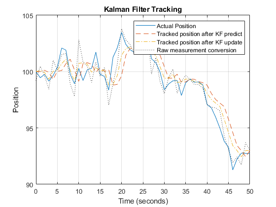
figure(2);
plot(time_line, X_a);
hold on;
grid on;
plot(time_line, X_p, '--');
plot(time_line, X_u, '-.');
plot(time_line, X_m, ':', 'Color', 'k');
title('Kalman Filter Tracking');
xlabel('Time (seconds)');
ylabel('Position');
legend('Actual Position', 'Tracked position after KF predict', ...
        'Tracked position after KF update', 'Raw measurement conversion');